|
Analysis of Two Numerical
Variables with Stata |
The residuals are the errors of prediction that we perform within our
sample. Since for the cases of the sample we have the actual value
(Y) and the predicted value (∧Y), we can compute the residuals
e:
Analyzing the residuals we can determine if the regression is
appropriate to perform predictions, or if it has anomalies and we
should be careful with the results that we get.
We have to first compute the residuals for each point. We can do it
with:
predict exam_res, residuals
The residuals of the regression is just a numerical variable for which
we can obtain the usual numerical and graphical descriptions. For
instance we can plot a histogram of the residuals:
histogram exam_res
This is the histogram that we get:
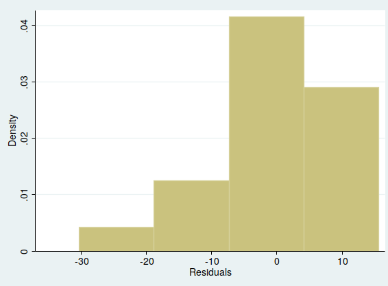
The residual histogram should look similar to the normal
distribution. If it is very different, then our regression would be of
bad quality. In this case since we have very few cases in our data
set, we can say that the histogram of the residuals is appropriate.
The other main graphical tools to analyze the residuals is the
residual diagram. It is a scatterplot between the residuals and the
explanatory variable. We can plot it with:
scatter exam_res MIDTERM, yline(0) title("Residual Diagram")
We have added a title with the "title" option. and a horizontal line
at 0 with "yline(0)", which is useful to assess the residuals, as
they should be distributed without any special pattern above and below
this horizontal line. This is the residual diagram:
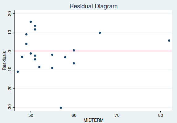
Given the small sample, the residual diagram does not show either any
special pattern, which is what we want for our regression to be able
to predict correctly.
File translated from
TEX
by
TTH,
version 4.08.