|
Analysis of Times Series with Stata |
|
1. Computing the trend with
moving averages |
To analyze times series with Stata, we have to declare that the
variable we want to analyze is of "time series" type.
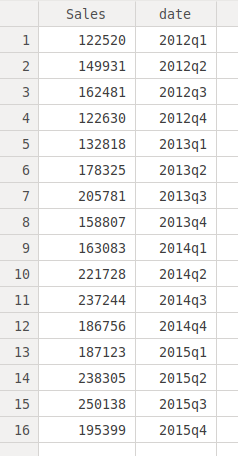
We will first import a data set on the sales of ice cream at an ice
cream shop during 4 years:
Dades sobre les vendes a una geladeria
Data is quarterly from the first quarter of 2012 until the fourth
quarter of 2016, that is, 16 quarters.
Import the data to Stata using the File - Import menu, remember to
tell Stata that the first row contains the name of the variable. There
is only one variable, "Sales", that has the time series that we want
to analyze.
We have to first define a variable called "date" that will contain
an indicator of time for each period. To do this, we give the
following commands to Stata:
generate date = tq(2012q1) + _n -1
format %tq date
This will generate a new varaible with an year/quarter indicator for
each case of the time series. If we look at the data window, we see it
as follows:
Now we have to tell Stata about the frequency of the time series. For
this, we declare the "Sales" variable as a times series according to
the "date" variable we have just created, with:
tsset date
We can first get the time series plot of "Sales". We do it with the command:
tsline Sales
The graph we obtain is:
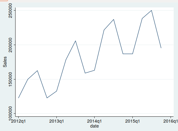
As it can be seen in the time plot, we can observe an increasing trend
and a strong seasonality. The series is below the trend during the
first and fourth quarters, and above the trend during the second and
third quarters.
To identify the trend, we start with the method of moving
averages. Considering that this is a quarterly series, and therefore
the frequency is even (4 quarters within a year), we will have to use
a centered moving average of order 4, so that the moving average gets
centered with the original series.
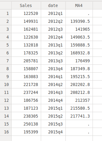
We first compute a moving average without centering and we put it at
the second case of each group of 4 consecutive cases used to compute
the mean:
tssmooth ma MA4= Sales, window(1 1 2)
replace MA4 = . in 1
replace MA4 = . in 15
replace MA4 = . in 16
The first commands computes the moving average. At the "window"
option it is set how the moving average should be computed. The first
number in the brackets says how many cases before the current case
will be used, the second one tells to include the current case in the
mean, and the third one how many cases after the current case are to
be used. Therefore, (1 1 2) tells Stata to compute an average using 4
cases, 1 before, the actual case, and 2 after, all consecutive. The
three other commands eliminate the first case and the last two cases,
since there is not enough information to compute a complete moving
average of order4. Now the data window looks as follows:
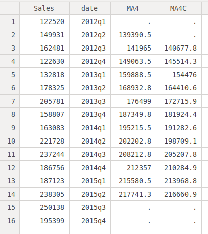
If the order of the moving average was uneven, we would stop
here. Considering it is even, we have to perform a second step, that
is, centering the moving average. To compute the centered moving
average we now compute the moving average of order 2 using the moving
average of order 4 we have already computed. We can do it with the command:
tssmooth ma MA4C = MA4, window(1 1 0)
replace MA4C = . in 2
replace MA4C = . in 15
The first command works as before, it is telling Stata to compute the
moving average, using MA4 which are the moving averages of order 4 we
computed previously, and including only the previous and the current
case (1 1 0). Line 2 and 3 eliminate the cases when there is not
enough information to compute the moving averages. The window looks
now as follows:
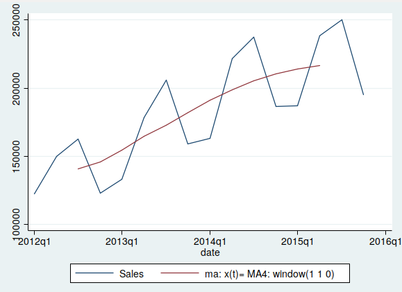
We already have the trend of the series. To confirm that it is really
the trend, we can now plot the original series together with the
trend. We can do it with the command:
tsline Sales MA4C
The graph is:
File translated from
TEX
by
TTH,
version 4.08.