<< Previous Index Next >>

Analysis of Times Series with Stata

2. Computing seasonal components and predicting with an additive series

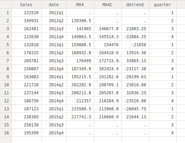
To compute the seasonal components we have to follow several steps. First, we have to eliminate the trend from the series, and next we have to eliminate the irregular component.

To eliminate the trend from the series we simply deduct the trend from the series:

generate detrend = Sales - MA4C

To eliminate the irregular component, we have to take a mean of the "detrend" variable we have just created within each quarter. To do this, we first generate a variable called "quarter" indicating the quarter:

gen quarter = quarter(dofq(date))

Let's see the variable we have created:

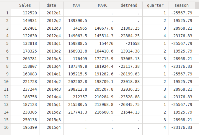
We now compute the seasonal components, by computing the mean over the quarters, which eliminates the irregular component:

bysort quarter: egen season = mean(detrend)
sort date

The first command computes the means by quarters, and the second one reorders the cases according to time since the first command disorders them.

If we know look at the quarters, we can see that we have same seasonal component for each quarter:

To confirm what we had seen at the time series plot, at quarters 1 and 4 the seasonal component is negative, so that the series is below the trend, while for quarters 2 and 3 the seasonal component is positive, the series is above the trend.

Suppose we want to predict the value of the series for the third quarter of 2016, that is 3 quarter into the future after the last quarter of 2015. We have to first compute a linear trend, and we can do it with the command:

. reg Sales date

      Source |       SS       df       MS              Number of obs =      16
-------------+------------------------------           F(  1,    14) =   21.34
       Model |  1.5120e+10     1  1.5120e+10           Prob > F      =  0.0004
    Residual |  9.9174e+09    14   708386771           R-squared     =  0.6039
-------------+------------------------------           Adj R-squared =  0.5756
       Total |  2.5037e+10    15  1.6692e+09           Root MSE      =   26616

------------------------------------------------------------------------------
       Sales |      Coef.   Std. Err.      t    P>|t|     [95% Conf. Interval]
-------------+----------------------------------------------------------------
        date |    6668.61    1443.43     4.62   0.000     3572.761     9764.46
       _cons |   -1255019   311130.3    -4.03   0.001     -1922327   -587710.5
----------------------------------------------------------------------------

At the last two lines we can see the values for the constant and the slope of the linear trend. To obtain a prediction adjusted for seasonality, we have to first figure out the value of "date" for the quarter we want to predict. Stata codifies dates ("date" is our variable) with an internal number. To see the number corresponding to the third quarter of 2016, we enter:

di tq(2016q3)

Stata tells us that this number is 226. We now predict the trend for the third quarter of 2016:

. adjust date = 226

-----------------------------------------------------------------------------------
     Dependent variable: Sales     Command: regress
 Covariate set to value: date = 226
-----------------------------------------------------------------------------------

----------------------
      All |         xb
----------+-----------
          |     252087
----------------------
     Key:  xb  =  Linear Prediction

To adjust the seasonal component we first figure out its value for the third quarter, asking Stata to show us the value of "season" but only for the third quarter:

. list season if quarter == 3

     +----------+
     |   season |
     |----------|
  3. | 28968.21 |
  7. | 28968.21 |
 11. | 28968.21 |
 15. | 28968.21 |
     +----------+

And finally we obtain the prediction adjusted by the sesonality:

. di 252087 + 28968.21
281055.21

Sales of ice cream are predicted to be 281055.21 for the third quarter of 2016.

<< Previous Index Next >>

File translated from T_EX by T_TH, version 4.08.