| Analysis of Times Series with Stata |
| 3. Computing seasonal components and predicting with a multiplicative series |
generate temps = tq(2012q1) + _n -1
format %tq temps
tsset temps
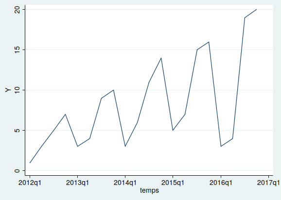
We now obtain the times series plot:
tsline Y

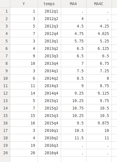
generate detrend = Y/MA4C
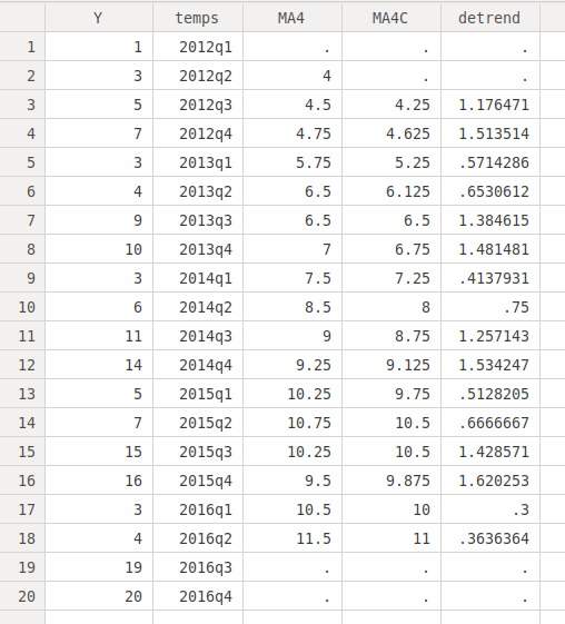
gen quarter = quarter(dofq(temps))
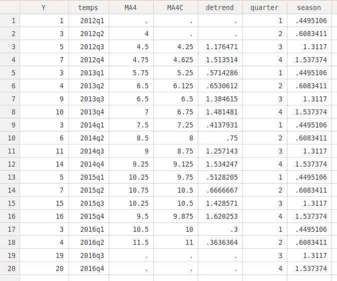
bysort quarter: egen season = mean(detrend)
sort temps
. reg Y temps

      Source |       SS       df       MS              Number of obs =      20
-------------+------------------------------           F(  1,    18) =   11.39
       Model |  244.830451     1  244.830451           Prob > F      =  0.0034
    Residual |  386.919549    18  21.4955305           R-squared     =  0.3875
-------------+------------------------------           Adj R-squared =  0.3535
       Total |      631.75    19       33.25           Root MSE      =  4.6363

------------------------------------------------------------------------------
           Y |      Coef.   Std. Err.      t    P>|t|     [95% Conf. Interval]
-------------+----------------------------------------------------------------
       temps |   .6067669   .1797891     3.37   0.003     .2290441    .9844897
       _cons |  -123.7218   39.11786    -3.16   0.005    -205.9054   -41.53823
------------------------------------------------------------------------------
And now we figure out the value of the time variable for the third quarter of 2017:
. di tq(2017q3)
230
We now obtain the prediction for the trend for the third quarter of 2017:
. adjust temps = 230

-----------------------------------------------------------------------------------
     Dependent variable: Y     Command: regress
 Covariate set to value: temps = 230
-----------------------------------------------------------------------------------

----------------------
      All |         xb
----------+-----------
          |    15.8346
----------------------
     Key:  xb  =  Linear Prediction
We check the value of the seasonal component for the third quarter:
. list season if quarter == 3

     +--------+
     | season |
     |--------|
  3. | 1.3117 |
  7. | 1.3117 |
 11. | 1.3117 |
 15. | 1.3117 |
 19. | 1.3117 |
     +--------+
And we obtain the prediction adjusted by the trend, notice that we now multiply the seasonal component:
. di 15.8346*1.3117
20.770245
It is predicted that "Y" will have a value of 20.770245 at the third quarter of 2017.